Table of Contents

1       Accuracy and precision
1.1    Calibration error
1.2    Random error
1.3    Blunder error
1.4    Combined error, error budget
2       Notes on error measures and their interrelation
3       Preparations for accuracy/precision evaluations of GPS positions using NAVGEN
4       The NAVGEN Algorithm
4.1    History
4.2    Descriptions of the NAVGEN Algorithm
4.3    Implemented NAVGEN Algorithm

1. Accuracy and Precision

When talking about measurement errors at least the following types of error have to be distinguished:

1.1 Calibration error

In Germany we have a saying: ‘To measure means to compare’. When you measure a length, using a yardstick you are actually comparing the length to the wavelength of light, which latter is defined as the standard for the dimension of length. As this is not a very practical procedure, you use a tool, the yardstick. No tool is perfectly calibrated, so the tool introduces an error in the measurement. A zero offset in a measurement tool introduces a constant calibration error for all measurements in the series, whereas a constant error in the scale divisions of the yardstick introduces an error, which is proportional to the length measured. The calibration error can be determined by using a more accurately calibrated tool and can be cancelled or minimized in this way. The calibration error is also called  'Systematical Error' or 'Bias'.  If  a measurement  has a small calibration error , it has a 'high accuracy'.

1.2 Random error

1.2.1 Description and determination

If you measure the height of the same person with a yardstick 100 times or so, you will probably get data that differ by a few millimeters. Provided the yardstick is perfectly calibrated and the height of the person does not change during the measurements, this error is caused by inaccuracies in the individual readings. In the normal case, half the readings will be too short, half will be too long. If one takes the deviations from the mean measurement, these values are the random errors following a Gaussian or Normal Distribution.

In the case of position determination you actually determine two quantities, the latitude and the longitude. These two quantities are measured in degrees (and fractions thereof). For the determination of the position error in distance the measurements have to be converted from degrees to metres. The resulting values are usually called Northings and Eastings. The random errors in distance can be determined if a large number of measurements are made on a fixed position, and by determining the individual deviations of the northings and eastings from their mean values.

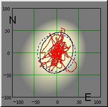
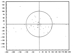
1.2.2  Scatter plot and random walk

If the random errors are plotted in an x/y diagram then the data will produce either a Scatter Plot (Fig. 1) or a Random Walk (Fig.2) In a scatter plot the individual errors are (seemingly) independent of each other. A random walk suggests residual systematic errors, e.g. caused by small unnoticed variations in the satellite ephemeridis,  by path variations of the transmitted signals in the ionosphere, or by deliberate data manimulation. Such a random walk necessitates a longer measurement/averaging period and further statistical treatment (decorrelation) of the random errors (c.f. Autocorrelation function).

Fig. 1 : Scatter plot	Fig. 2 : Random walk

1.2.3 The generation of the error contour

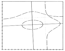
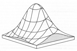
The scatter plot or the random walk is the first graphical representation of the measured positions.  Both provide qualitative (but no quantitative) indications of the measurement accuracy.  As a first statistical evaluation we calculate the probability density functions for the deviations of the fixes in both coordinate system axes from the mean position (Fig.3).  If we put these functions upright with the PD axis pointing in the z direction,  a 3d PDF surface will be generated, the 'mound' as shown in Fig. 4. From the mound we can obtain error contours for a defined probability content, by 'cutting off' the top of the mound at a certain height (the required probability). The resulting genuine error contour is an ellipse in the general case, or a circle in the special case that both standard deviations are equal. In this way, we can generate an error ellipse for any desired probability level. (This however requires complicated integration of a two-dimensional elliptical integral.  Error ellipse integration calculation: Pdf, mcd file.)

Fig. 3: PDF functions in orthogonal axes	Fig. 4: 3d PDF function

Error ellipses as an error contour are not very practical for navigation, as five parameters are needed for their description, the origin, the length of each semi-axis and the orientation (e.g. angle between the major semi-axis and the x-axis.  A more handy contour is a circle, which is fully described by the origin and the radius.  In the case of error contours, an additional parameter is the 'confidence content', i.e.  the probability that a measured position lies within the contour.  (For a sufficiently large number of position fixes the probability should be equal to the percentage of fixes lying inside the contour.)  In navigation we usually require a probability of 0.95, i.e. 95%.

The only measure for navigation errors that provides a fixed probability is the 'Circular Error Probability' , the CEP value, to which usually an index indicating the probability is added. (Other error measures, such as dRMS or 2dRMS do not provide a predefined probability.)  

Sometimes the Rayleigh PDF is used as an approximation for the bivariate distribution of navigation errors. A pre-requirement for this approximation are equally distributed and uncorrelated errors in both coordinates. As can be seen in the chapter below, this assumption is not always true,  particularly with GPS measurements in the order of  the correlation time. The NAVGEN algorithm, however, provides a consise calculation of CEP errors.

If a position measurement has a small error circle, it is  a 'high precision' measurement. 

1.2.4 The influence of the number and time spread of the measurements

One-dimensional statistics teaches us that the standard deviation depends on the sample size, i.e. the number of measurements taken. As NAVGEN is based on the standard deviations of the Northings and Eastings, the error quantities (dRMS and CEP) depend on the number of measurements taken. In order to keep NAVGEN calculations compatible with each other, the author recommends to sample data with a rate of 1/s for at least 24 h (86,400 data sets). 

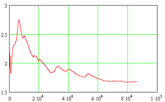
Fig. 4 below illustrates the decrease in  RMS position error as a function of the number of samples or the measurement time. Due to the time-dependent random walk the term time should be more correct (see also Autocorrelation function).

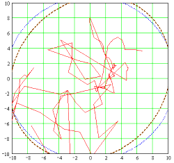
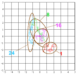
The effect of shorter measurement time than 24 hours is illustrated in  Fig. 5. It shows a coordinate grid with the 24-h  mean position in the centre (0/0). From the 24 h data set 4 one-hour subsets were processed starting at 0 hours, 8 hours, 16 hours, and 24 hours.  For each subset the position fixes' random walk and the 95% error ellipse are shown. The figure clearly demonstrates that sampling times, even in the order of one hour (3600 data sets), could yield a position offset of up to 2 m  from to the 24-hour mean position. This offset does not only depend on the sample size, but is obviously also time-dependent.

Fig. 5 also shows that short-time measurements (in the order of one hour)  can deviate quite strongly from a circular distribution (in which cases the use of the Rayleigh distribution is not  justified).

Fig. 4: RMS error over samples/ time	Fig. 5: Small sample measurement errors

1.2.5 Autocorrelation function

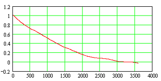
The autocorrelation function shows the strength of correlation between the errors of successive position fixes. Such a correlation will result if successive fixes are not statistically independent from each other, but follow a certain pattern such as a random walk. The correlation factor drawn on the vertical axis of the diagram (Fig. 6) could vary between one and zero or even become negative. On the horizontal axis the data spacing is drawn. In this particular case the spacing is the time difference in seconds. The graph below has been derived from the GPS data set recorded on 16 September 2006. It shows an exponential decay with a time constant τ of approx. 20 minutes. If we accept a residual correlation of ≤ 5 % (3τ) as sufficient statistical independence, then GPS data should be sampled not faster than once every hour. Of such data a sufficient number would be required to arrive at a statistically reasonable statement for the navigation error. Such a measurement would take several days. The NAVGEN algorithm follows another avenue and mathematically decorrelates the collected data, so that the measurement period can be shorter.

Fig. 6 : Autocorrelation function

1.3 Blunder error

The blunder error is a coarse error caused by the user, e.g. by permutation of decimals when writing down measurement values. This error is unpredictable and will not be considered any further here.

1.4 Combined error, error budget

When we are talking of measurement accuracy, then we usually mean the overall measurement error, i.e. the combination of the calibration error and the random error. In order to predict or determine the accuracy of a technical system, an error budget can created in which all known error contributions are listed with their magnitudes. The root mean square (RMS) value of all these is normally conceived as the measurement accuracy of the system.

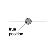
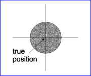
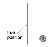
The calibration error is also called the 'Systematical Error' or 'Bias' and the random error the 'Precision' of the measurement. The following diagram (Fig. 7) shows the relationship between accuracy and precision.

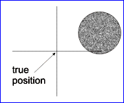high accuracy, high precision	high accuracy, low precision	low accuracy, high precision	low accuracy, low precision
Fig. 7 : Accuracy and Precision

2. Notes on error measures and their inter-relation

2.1 Probable error, standard error, standard deviation (PE, SE, SD, σ)

One-dimensional errors that follow a Gaussian distribution  are characterized by the 'Probable Error (PE)' in statistical terms also called the 'Median' having a confidence level of 50%. Half of the errors are larger, half of the errors are smaller than the probable error.  Another error measure is the 'Standard Error' (SE) or 'Standard Deviation' (SD or σ ), having a confidence level of 68.3 %. Often the higer confidence  multiples  2σ  (95.5 %) or 3σ  (99.7 %) are used. One-dimensional error statistics plays an important role in the determination of the position error, as it is applied to the measurement errors of the individual position coordinates. The standard deviations (SD) of these serve as the input to most further calculations.  

2.2 Axes of the error ellipse

From the random errors of the Northings and Eastings the error ellipse can be calculated.  For this purpose it is necessary to de-correlate the errors first. The de-correlation is achieved by  'turning' the data set  by an angle that  follows from the correlation factor.  New standard deviations are calculated from the de-correlated data set. The basic error ellipse  is described by the standard deviations of the de-correlated former Northings and Eastings and  by the turning angle (Fig. 2 above). This ellipse has a confidence content of 39.3 %.  If both standard deviations are multiplied by the factor of  1.177 (2.449),  then the confidence content is 50%  (95%).  The confidence content can be calculated  using the Mathcad Ellipse sheet  (pdf / mcd).

2.3  Distance Root Mean Square (dRMS )

Distance Root Mean Square (dRMS) is a measure which is relatively easy to determine.  There are two ways to determine dRMS:
(i)  For each measurement the error vector magnitude, i.e. the distance from the measured position to the mean position, is  determined.  dRMS is then the standard deviation of these error values.
(ii)  For both, Northings and Eastings, the standard deviations (SDs) are determined. dRMS is then the root of the sum of the squared SDs.

Unlike with the one-dimensional SD, dRMS error probability is not fixed, but varies between 63.2% and 68.3%, depending on the ratio between the SDs of the Northings and the Eastings (the larger to be used as the denominator), see Tab. 1 below.
Besides dRMS  the multiple 2DRMS is used, providing confidence levels that vary between 95.5 % and 98.2 %, see Tab. 1 below.

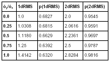Tab. 1: Probabilities of dRMS and 2dRMS

2.4  Circular Error Probability (CEP)

The genuine 2D error contour of positioning errors  is an ellipse, as described in chapter  1.2.3 above.  The dRMS values and their multiples generally do not provide a fixed confidence level. CEP  is a conversion of the error ellipse to a circle of a per-determined and fixed probability content.

CEP without an index or suffix is called the 'circular error probable'. The value provides the radius of  a circle about the mean position with a confidence content of 50%. Other indices or suffixes provide a radii with the respective 'circular error probabilitiy', e.g. CEP95.

The accurate calculation of CEP is quite intricate, as de-correlated standard deviations for  the two coordinates are required and the two-dimensional probability integral (pdf / mcd) has to be solved (or tabulated values have to be used) to determine the CEP radius. There are also existing approximations for the CEP radii, which in the past were often used with the non-decorrelated standard deviations of the Northings and Eastings. Due to the processing power generally available today, these approximations shall not be discussed here. NavGen is providing the accurate solution, anyway.

3 Preparations for accuracy/precision evaluations of GPS positions

Your measurement set-up should satisfy the following requirements:

4   The NAVGEN Algorithm

4.1  History

In the early 1980s the author started to look into the matter of navigation accuracy. At that time various navigation and positioning systems were in use, such as:

As numerous as the systems were the accuracy statements.  For various statements such as 'repeatable accuracy' there was no generally accepted definition nor method of determination, nor probability level. In so far it was difficult, if not impossible, to  compare accuracies of different systems.

After some research, the author came to the conclusion that only one already existing term made sense to be used : the Circular Error Probability (CEP).

In the preparation of the NAVGEN algorithm the following scientific and technical papers were resorted to:

The theory contained in these reports, however, cannot be used directly - not least as certain data need to be looked up in diagrams. The NAVGEN algorithm overcomes these shortcomings by means of interpolation polynoms.  NAVGEN  provides a concise calculus for determining accuracy/precision of static navigation data using an input table of collected position fixes.

4.2  Descriptions of the NAVGEN algorithm

The NAVGEN algorithm is described in the following technical papers:

Harre, Ingo: A Standardized Algorithm for the Determination of Position Errors
by the Example of GPS with and without 'Selective Availability;
International Hydrographic Review, Vol. 2, No. 1 (New Series), June 2001.

Harre, Ingo: Accuracy Evaluation of Polar Positioning Systems Taking
POLARFIX as an Example; International Hydrographic Review, No. 1, 1990.

Harre, Ingo: Modellieren von Navigationsfehlern – Fehlertypen und
Entwicklung eines Fehlerkreismodells; Ortung & Navigation, No. 3, 1987.

Harre, Ingo: Positionsgenauigkeiten von Navigationsverfahren; Ortung &
Navigation, No. 3, 1980.

4.3 Implemented NAVGEN algorithm

The NAVGEN algorithm, as realised in   MATHCAD® , can be downloaded and studied here in form of a PDF file and here as a MATHCAD file.